Mathematical Model UNTRIM2
From BAWiki
Short Description
The numerical method UNTRIM2 is closely related with its predecessors UNTRIM and UNTRIM2007. UNTRIM2 is a semi-implicit finite difference (-volume) model, based on the three-dimensional shallow water equations as well as on the three-dimensional transport equation for salt, heat, dissolved matter and suspended sediments. The essential, main and revolutionary difference, is due to the sub grid technology used to discretise bathymetry with much finer resolution compared to the computational grid.
Sub Grid Technology
Computational Grid and Sub Grid
- Computational Grid:
- UNTRIM2 is able to work on unstructured orthogonal grids (UOG). The modelling domain is covered by a grid consisting of a set of non-overlapping convex polygons, usually either triangles or quadrilaterals. The grid is said to be an unstructured orthogonal grid if within each polygon a point (hereafter called a center) can be identified in such a way that the segment joining the center of two adjacent polygons and the side shared by the two polygons, have a non-empty intersection and are orthogonal to each other.
- Sub Grid:
- Model bathymetry is defined with sub grid resolution. Sub grid resolution can be much finer compared to the resolution of the computational grid.
- Non-Linearities:
- Water volume within a polygon may be non-linearily dependent on water level.
- Flow area along edges may also become non-linearily dependent on water level.

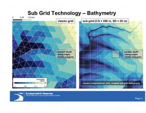
In Figure Tidal Flats Elbe Estuary the discrete model bathymetry for the classical grid (left) as well as for the case using sub grid technology (right) is displayed. In the classical case, e.g. for a triangular unstructured grid, depth is constant within polygons as well as along edges.With use of sub grid technology many more details of bathymetry become visible. This is mainly due to the fact, that depth is allowed to vary within a polygon as well as along edges. Therefore, also small topographic structures can be represented in the model bathymetry.
Computational Results
Water level as well as current velocity are computed on the (coarse) computational grid only, but not on the (much finer) sub grid. Typically water level corresponds to the mean value within a computational polygon. And current velocity is equivalent to the mean velocity for the respective actual flow area along an edge.

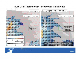
In Figure Synoptic current velocity for a tidal flat area in the Elbe Estuary, computed current velocity for the classical grid is shown on the left, whereas results obtained for a grid using sub grid bathymetry are displayed on the right. In the classical case any polygon is either completely wet or dry. In the sub grid case instead, any polygon, and also any edge, may become also partially wet. This feature is mainly responsible for the quasi-natural flooding obtained with sub grid technology, where water is enabled to penetrate more rapidly along the deep tidal channels.
Benefits
- Bathymetry can be prescribed independent of computational grid resolution.
- Accuracy is, in principle, only limited due to measurement errors of bathymetric data.
- For any water water level, modelled water volume is very close to the natural water volume. Similar is true for the flow area.
- Dry and wet areas can be prescribed in great detail.
- Comparable accuracy with respect to bathymetry can be achieved at much lower CPU cost using sub grid technology, compared to a full discretisation of bathymetry with the classical grid approach.
Physical Processes
- reynolds-averaged Navier-Stokes equations (RANS)
- local acceleration (inertia)
- advective acceleration
- Coriolis acceleration
- barotropic pressure gradient
- baroclinic pressure gradient
- hydrostatic or non-hydrostatic pressure
- horizontal turbulent viscosity
- vertical turbulent viscosity influenced by density stratification
- bottom friction
- wind friction
- sources and sinks
- horizontal acceleration due to wave effects (by means of radiation stress)
- transport of tracers
- local rate of change of concentration
- advective rate of change of concentration
- optional flux limiter : Minmod, van Leer or Superbee
- horizontal turbulent diffusivity
- vertical turbulent diffusivity influenced by density stratification
- settling of particles, deposition and erosion (for suspended sediments)
- heat-transfer to/from the atmosphere and to/from the bottom
- sources and sinks
- sinks with immediate return inflow at a different location, with optional modification of inflow-temperature as well as -salinity
Computational Results
- water level elevation at the free surface
- current velocity
- tracer concentration (e.g. salinity, temperature, suspended sediments)
- hydrodynamic pressure
Note: when UNTRIM2 is used in two-dimensional (depth-integrated) mode, results correspond to the depth-averaged values for the above-mentioned quantities.
Publications
- Casulli, V. (2008), A high-resolution wetting and drying algorithm for free-surface hydrodynamics, International Journal for Numerical Methods in Fluids, Volume 60, Issue 4, pages 391 - 408. See abstract.
- Casulli, V. and Stelling, G. S. (2010), Semi-implicit sub grid modelling of three-dimensional free-surface flows, International Journal for Numerical Methods in Fluids. See abstract.
- Sehili, A., Lang, G. and Lippert, C. (2014), High-resolution subgrid models: background, grid generation, and implementation, Ocean Dynamics, Volume 64, Issue 4, pages 519 - 535. See abstract.
Presentations
- IZW-Campus (Podcast, available in German only)
- 2020-06-16: UnTRIM - UnTRIM und seine Vorgänger.
- Latest Presentation:
- Neue Möglichkeiten in der Ästuarmodellierung (in German only), slides, September 22, 2011, approx. 3.7 MB.
- Gittergenerierung für UnTRIM2 (in German only), slides, September 22, 2011, approx. 4.1 MB.
- Older Presentations:
- An Overview of the Numerical Method within UnTRIM, slides, August 23, 2011, approx. 1.2 MB.
- An Overview of the Numerical Method within UnTRIM2, slides, August 24, 2011, approx. 1.8 MB.
- Further Experiences using Sub Grid Technology, slides, May 10, 2011, approx. 11 MB.
- UNTRIM2 (sub grid) at BAW Hamburg, slides, November 11, 2010, approx. 15 MB.
R&D Projects
- UnTRIM SubGrid-Topografie (2009-2011)
- final report, approx. 4.3 MB.
Other Users
Different versions of the computational core UnTRIM2 developed by Prof. V. Casulli are used at the following organizations:
- Delta Modeling Associates, Inc., San Francisco, California, USA
- Resource Management Associates, Fairfield, California, USA
- University of California, Davis, California, USA
- Virginia Institute of Marine Science, Gloucester Point, Maryland, USA
Similar Software
Not existing so far.
Validation Document
Not available.
User Interface Description
This document contains a detailed description of all interface functions and routines available to the user. The following topics are dealt with in this document:
- set data (set-interfaces),
- get data (get-interfaces),
- check grid consistency as well as accuracy of iteratively computed results (check-routines),
- external routines called by the computational core (user-interface-routines) which are required to,
- define paths and names of the standard input data files, to
- define (set) the inital state (initial data), to
- set the forcing terms (e.g. along open boundaries) for each time step, and to
- retrieve the computational results.
- tables with short descriptions of all get- and set-interfaces available, and
- example standard input data files.
A PDF-version of the user interface description document is freely available for download:
- Latest version:
- UNTRIM2 (edition 2010) user interface description (in Englisch, ca. 740 kB)
- Earlier versions:
- UNTRIM2 (edition 2009) user interface description (in Englisch, ca. 1.4 MB)
MPI-Parallelisation
Not realised.
BAW-Specific Informations
Grid Generation
An unstructured orthogonal grid for UNTRIM2 can be prepared using JANET grid generator software, made by SmileConsult. For further informations related to the integration of JANET into BAW's programming environment please visit JANET program description.
Simulation
The mathematical model UNTRIM2 is partially integrated into BAW's programming environment. More detailed information concerning it's integration can be found visiting UNTRIM2 program description.
Graphical Presentation of Computed Results
To display UnTRIM2 results currently several methods are used at BAW. The more important ones are,
- NCPLOT, for data available throughout the computational domain,
- VVIEW2D and/or LQ2PRO, for data at longitudinal- and/or cross-sections, as well as
- GVIEW2D, for data at specific Locations,
- QUICKPLOT for data available throughout the computational domain.
Analyses of Computational Results
A great variety of methods for analyses of computational results is available which enables the user to respond to many different questions. The following methods are currently available:
- NCANALYSE for computation of characteristic numbers (tide-dependent, independent of tides).
Coupling to Independent Sub-Models
Not realised.
back to Mathematical Models for Coastal Areas and Estuaries
