TAYLORTARGETDIAGRAM: Difference between revisions
From BAWiki
mNo edit summary |
Günther Lang (talk | contribs) working group POS |
||
| (One intermediate revision by one other user not shown) | |||
| Line 3: | Line 3: | ||
|name=taylorTargetDiagram | |name=taylorTargetDiagram | ||
|version=May 2019 | |version=May 2019 | ||
|version_descr= | |version_descr=September 2022 | ||
|catchwords= | |catchwords= | ||
Taylor-Diagram<br /> | Taylor-Diagram<br /> | ||
| Line 23: | Line 23: | ||
<gallery> | <gallery> | ||
Taylor.png |Example picture Taylor diagram | Taylor.png |Example picture Taylor diagram | ||
Target.png| Example picture Target diagram | Target.png | Example picture Target diagram | ||
TaylorTargetTable.png |Example picture of the resulting table | |||
</gallery> | </gallery> | ||
| Line 40: | Line 40: | ||
* Number of data points used for the comparison | * Number of data points used for the comparison | ||
<br /> | <br /> | ||
|inputfiles= | |inputfiles= | ||
| Line 55: | Line 48: | ||
# Taylor-Diagram as bitmap (*.JPG,*.PNG), as a vector graphic (*.PDF,*.EPS) or as a MATLAB figure file (*.FIG). | # Taylor-Diagram as bitmap (*.JPG,*.PNG), as a vector graphic (*.PDF,*.EPS) or as a MATLAB figure file (*.FIG). | ||
# Target-Diagram as bitmap (*.JPG,*.PNG), as a vector graphic (*.PDF,*.EPS) or as a MATLAB figure file (*.FIG). | # Target-Diagram as bitmap (*.JPG,*.PNG), as a vector graphic (*.PDF,*.EPS) or as a MATLAB figure file (*.FIG). | ||
# (optional) Table of the model performance quantities (*. | # (optional) Table of the model performance quantities (*.XLS) | ||
# (optional) Text file with meta-information (*.TXT). | # (optional) Text file with meta-information (*.TXT). | ||
| Line 69: | Line 62: | ||
|language=[[MATLAB]] | |language=[[MATLAB]] | ||
|add_software= Linux: MATLAB Compiler Runtime MCR R2015a in directory /usr/local/MATLAB/R2015a | |add_software= Linux: MATLAB Compiler Runtime MCR R2015a in directory /usr/local/MATLAB/R2015a | ||
|contact_original= | |contact_original=U. Schiller, J. Benndorf, C. Rasquin | ||
|contact_maintenance=[mailto: | |contact_maintenance=[mailto:pos.proghome@baw.de Working group POS] with U. Schiller, J. Benndorf and C. Rasquin | ||
|documentation= Taylor, Karl E. (2001) "Summarizing multiple aspects of model performance in a single diagram". Journal of Geophysical Research, Vol 106, No. D7, April 16, 2001, Pages 7183 - 7192.<br /> | |documentation= Taylor, Karl E. (2001) "Summarizing multiple aspects of model performance in a single diagram". Journal of Geophysical Research, Vol 106, No. D7, April 16, 2001, Pages 7183 - 7192.<br /> | ||
Jolliff et al. (2009) “Summary diagrams for coupled hydrodynamic-ecosystem model skill as-sessment”. Journal of Marine Systems. Vol 76, Issues 1–2, 20 February 2009, Pages 64-82, ISSN 0924-7963<br />Siehe auch unter [[MATLAB]]. | Jolliff et al. (2009) “Summary diagrams for coupled hydrodynamic-ecosystem model skill as-sessment”. Journal of Marine Systems. Vol 76, Issues 1–2, 20 February 2009, Pages 64-82, ISSN 0924-7963<br />Siehe auch unter [[MATLAB]]. | ||
Latest revision as of 11:13, 6 September 2022
Basic Information
Name of Program
taylorTargetDiagram
Version-Date
May 2019
Description-Date
September 2022
Catchwords
Taylor-Diagram
Target-Diagram
model accuracy
comparison of model and measurement
CF NetCDF format
MATLAB
Acknowledgement: This project took advantage of netCDF software developed by UCAR/Unidata (www.unidata.ucar.edu/software/netcdf/).
Short Description of Functionality
The application taylorTargetDiagram (see also taylorTargetDiagram.dat) allows to visualize variables for the estimation of model performance (e.g. calculated by NCDELTA) as taylor and target diagrams and list them as table.
This Program is a further development of TAYLORDIAGRAM.
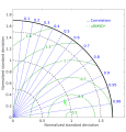
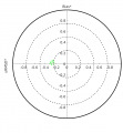
In the Taylor-Diagram standard deviation, correlation as well as pattern root mean square error (PRMSE) between reference and variant (e.g. model and observation) are graphically displayed. The target diagram shows the centered root-mean-square deviation and the bias. The combined presentation of the statistical characteristics of different physical quantities and locations in one diagram is possible. The statistical characteristics at different locations can also be combined to a mean value. As reference and variant values for the calculations of differences and statistcs results of different simulations or analyses as well as comparisons between measurements and model results may be used.
-
Example picture Taylor diagram
-
Example picture Target diagram
-
Example picture of the resulting table
In addition to the figures, a table including the following statistical values can be generated:
- Root Mean Square Error (RMSE)
- Taylor Skill 4 (Equation 4 in Taylor (2001))
- Taylor Skill 5 (Equation 5 in Taylor (2001))
- Centered Root-Mean-Square-Difference
- Bias (deviation of the mean values)
- Mean values of reference and variant parameters
- Standard deviation of reference and variant parameters
- Correlation between reference and variant parameters
- Attributes of the locations of the parameters compared in NCDELTA (cartesian and geographic coordinates, depth, location name)
- File name of the output file of NCDELTA
- Number of data points used for the comparison
Input-Files
- general input information (file type taylorTargetDiagram.dat);
- NCDELTA-Output files format (cf-netcdf.nc).
Output-Files
- Taylor-Diagram as bitmap (*.JPG,*.PNG), as a vector graphic (*.PDF,*.EPS) or as a MATLAB figure file (*.FIG).
- Target-Diagram as bitmap (*.JPG,*.PNG), as a vector graphic (*.PDF,*.EPS) or as a MATLAB figure file (*.FIG).
- (optional) Table of the model performance quantities (*.XLS)
- (optional) Text file with meta-information (*.TXT).
Methodology
The necessary statistical characteristics are read with MATLAB from NCDELTA result files and are visualized. The switch „With_Taylor_Diagram_Data=true“ has to be set to "true" in NCDELTA.DAT so that the required statistical values are included in the cf-netcdf-file written by NCDELTA.
The visualization of model accuracy in the taylor diagram is done according to Taylor (2001).
The visualization of model accuracy in the target diagram is done according to Jolliff et al. (2009).
Program(s) to run before this Program
Program(s) to run after this Program
MATLABFIGVIEWER, Excel
Additional Information
Language
Additional software
Linux: MATLAB Compiler Runtime MCR R2015a in directory /usr/local/MATLAB/R2015a
Original Version
U. Schiller, J. Benndorf, C. Rasquin
Maintenance
Working group POS with U. Schiller, J. Benndorf and C. Rasquin
Documentation/Literature
Taylor, Karl E. (2001) "Summarizing multiple aspects of model performance in a single diagram". Journal of Geophysical Research, Vol 106, No. D7, April 16, 2001, Pages 7183 - 7192.
Jolliff et al. (2009) “Summary diagrams for coupled hydrodynamic-ecosystem model skill as-sessment”. Journal of Marine Systems. Vol 76, Issues 1–2, 20 February 2009, Pages 64-82, ISSN 0924-7963
Siehe auch unter MATLAB.
- Example files:
- Example files can be found in $PROGHOME/examples/taylorTargetDiagram/
- A presentation with further examples and information can be found in $PROGHOME/examples/taylorTargetDiagram/_doc
back to Program Descriptions


